Lecture Notes UCU-TTS. Lecture 2. Vocoders and Modern TTS

Introduction to vocoders

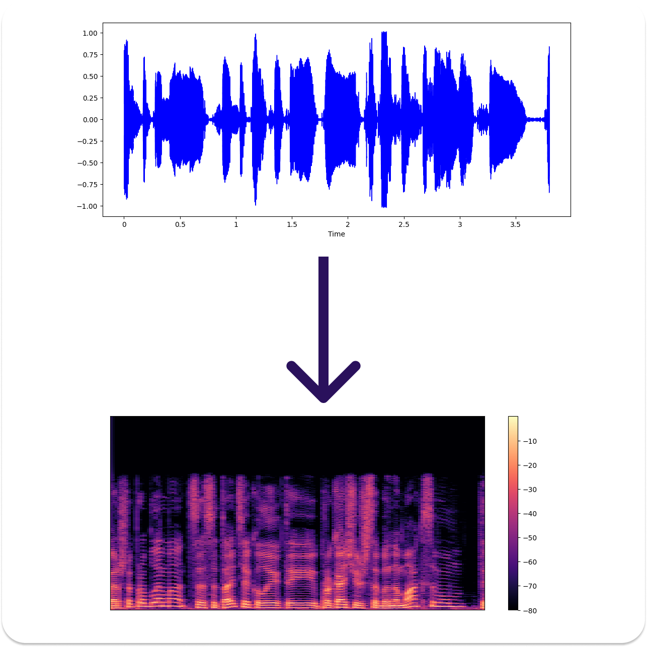
Most modern TTS systems, are in fact text-to-spectrogram systems. And once we obtained a spectrogram, more precisely a power spectrogram, we need a way to map it to the corresponding waveform. So Vocoders are spectrum to waveform models, and their primary task is to reconstruct the missing phase information, and we can think of them as inverse-spectrogram models.

\[\begin{align*} V: \mathbb{R}^{\text{F} \times \text{T}} \rightarrow \mathbb{R}^{\text{S}} \end{align*}\]

In case our TTS models outputs are not STFT-spectrograms but MEL-spectrograms, then task of vocoder is getting harder than merely phase reconstruction. But still we can think of this class of models as those that a given an arbitrary incomplete spectrum representation of the signal and are tasked to produce it’s corresponding time-domain representation.

[!Question] If you are given a complex valued STFT spectrogram $\text{Spectro} \in \mathbb{C}^{\text{F} \times \text{T}}$, how would you obtain a corresponding time-domain waveform $W \in \mathbb{R}^{\text{S}}$?

Griffin-Lim classic and simple approach for phase reconstruction was used in tacotron¹ paper. The proposed method starts with randomly initialized phase and runs a series of $STFT-iSTFT$ operations with fixed input spectrum magnitude and iteratively refined phase.

[!reminder] In polar notation complex numbers are represented as $z=re^{i\varphi}$

# adapted from: https://github.com/rbarghou/pygriffinlim

import librosa
import numpy as np
from IPython.display import display, Audio

def griffin_lim(spectrogram, n_iter=32, approximated_signal=None, stft_kwargs={}):
    _M = spectrogram
    for k in range(n_iter):
        if approximated_signal is None:
            _P = np.random.randn(*_M.shape)
        else:
            _D = librosa.stft(approximated_signal, **stft_kwargs)
            _P = np.angle(_D)

        _D = _M * np.exp(1j * _P)
        approximated_signal = librosa.istft(_D, **stft_kwargs)
    return approximated_signal

stft_kwargs = {'n_fft' : 2048}

audio_path = './data/LJ001-0051.wav'
waveform, sr = librosa.load(audio_path)

spectro = librosa.stft(waveform, **stft_kwargs)
spectro_mag = np.abs(spectro)

waveform_hat = griffin_lim(spectro_mag, stft_kwargs=stft_kwargs)

display(Audio(audio_path))
display(Audio(waveform_hat, rate=sr))

That said first valuable results in neural TTS modelling were obtained with very simple spectrogram to waveform inversion technique! Further adoption of Griffin-Lim was tampered with it’s applicability only to STFT spectrograms, when our aim is to process other spectral representations such as MEL-spectrograms, gamma-tones or any other signals represented in their spectral form.

Neural Vocoders

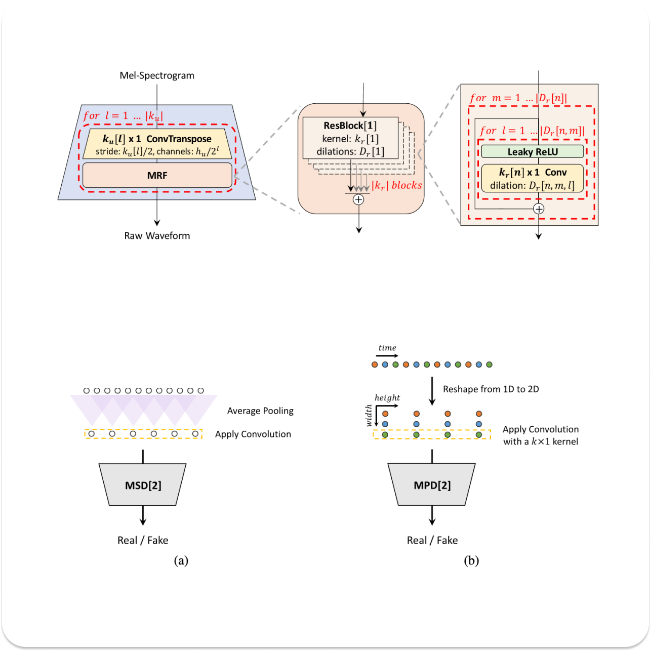
Vocoders have access to the whole spectrogram and intuitively they only need local information (few spectral frames) to do the spectrogram inversion. This allows us to run them in parallel, leveraging transposed-convolutions for temporal upsampling. HiFi-GAN² is fast and modern vocoder employing GANs to produce raw waveforms. This model effectively addresses local and global consistency via multi-period and multi-scale discriminators. Where multi-period discriminators sample points every [2, 3, 5, 7, 11] steps and is responsible for global consistency. In its turn multi-scale discriminator operates on raw audio, ×2 average-pooled audio, and ×4 average-pooled audio and is responsible for local consistency of the patches of various temporal resolutions.

Objective Metrics for TTS systems

In TTS modelling we care about both semantics and acoustics of the utterance. More specifically by semantics we mean preserved content and meaning of the phrase, and this aspect can be measured by computing WER on input text and transcripts obtained from generated utterances via separate ASR model. Low WER values signifies that semantic information was preserved by the model. By acoustic aspects of generated speech we mean proper prosody, preserved voice of the target speaker, room acoustics.

To measure acoustics properties of the generated speech we employ separate speaker recognition models like WavLM-TDNN³ and compute cosine similarity between real sample of the speaker and generated speech conditioned on voice-vector of the same speaker. Speaker similarity scores quantify ability of the TTS model in preserving of acoustical properties of the speech.

We can move further and measure similarity of prosody, by measuring FID⁴ between samples from real and synthesized distributions, the lower FID is the closer is prosody of synthesized sampled to real data. Another classic measure is Mean Cepstral Distortion(MCD).It’s aimed to measure distortions of acoustic information, this metric is widely used because it highly correlates with human perception. All metrics described above are neatly assembled in the repository for MQTTS⁵

Discrete Speech Representations

To bridge the gap and apply language modelling techniques to TTS field we need to obtain discrete representations for speech.

HuBERT

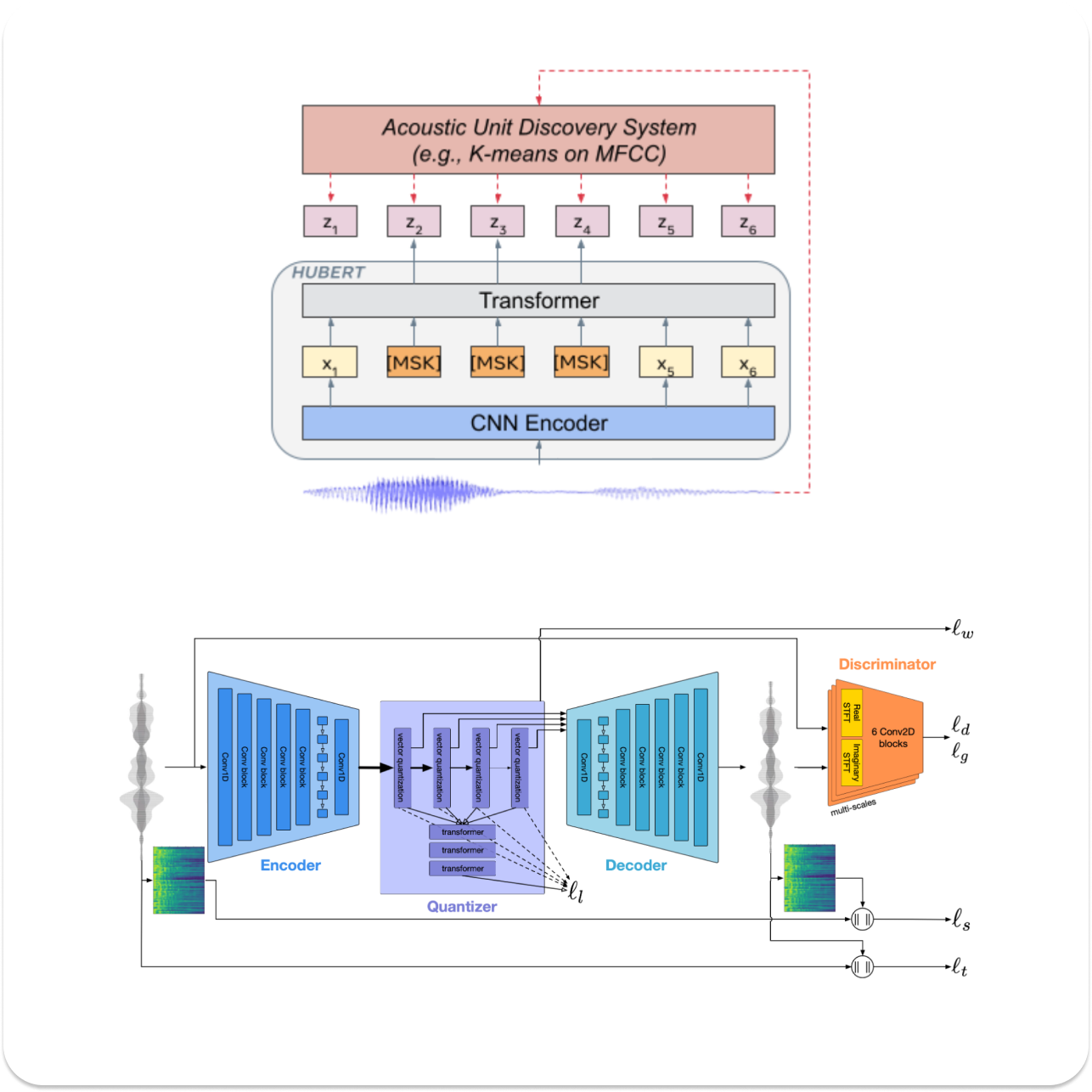
When it comes to semantics, we can leverage HuBERT⁶ a self-supervised model trained with masked language modelling objective. This model allows us to extract discrete tokens from input raw waveform. HuBERT is trained to reconstruct both masked and unmasked tokens with resulting loss function defined as: $L = \alpha L_{m} + (1 − \alpha)L_{u}$ , where $\alpha \in [0..1]$ is a hyper parameter that controls impact of each of the loss components. With $\alpha = 1$ shift focus towards learning language modelling capabilities, when $\alpha=0$ loss is computed only on unmasked tokens, that is similar to acoustic modelling.

HuBERT has no reconstruction objective, we can’t be sure that acoustic information is preserved in enough amount for applicability of these type of tokens for acoustic modelling. So what we obtain from the model is phone-like features, or data-driven neural-IPA-like phonemes! And this can be validated by training an ASR model with CTC-loss on top of the learned representations.

EnCodec

So we need a way to obtain acoustic tokens. EnCodec⁷ is a SOTA model that is trained to compress and tokenize speech signals into discrete units via Residual Vector Quantization (RVQ). EnCodec is trained to reconstruct inputs signals both in time-domain and spectral representations, additionally multi-scale discriminators are added to further improve quality of reconstruction.

Speech Tokenizer

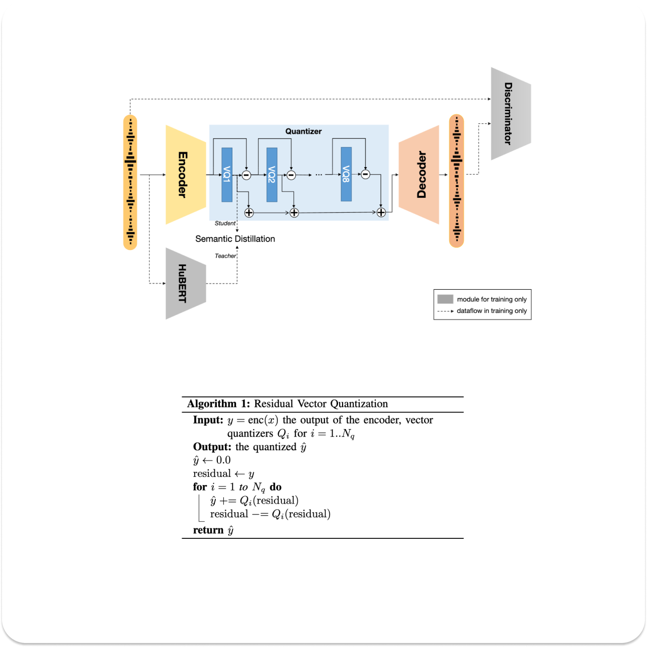
Now that we have both semantic tokens, that capture sequence modelling and text meaning, together with acoustic tokens that hold acoustic information we want to unify them and build a joint semantic-acoustic representation that can be leveraged for TTS modelling! That’s is precisely the idea of SpeechTokenizer⁸ , where HuBERT tokens are used for guided semantic residual quantization that allows to disentangle speech and store semantic information in the first quantizer $Q_{0}$ . Where all subsequent $Q-1$ qauntizers are responsible for preserving of acoustic information.

Whole pipeline is trained with both distillation and reconstruction objectives making SpeechTokenizer tokens suitable for downstream tasks as TTS. Bellow is definition of the distillation objective, that enforces similarity in each of the dimensions across all the time steps of the first quantizer features. This formulation intuitively facilitates long-range distillation constancy across all the timestep of the given utterance.

\[\begin{align*} L_{\text{distill}} = -\frac{1}{D} \sum_{d=1}^{D} \log \sigma(\cos(\text{AQ}^{(:,d)}, \text{S}^{(:,d)})) \end{align*}\]

[!Question] Speech Tokenizer disentangles content from acoustics, can you think of a way how would you further disentangle prosody or room characteristics?

Pheme

Language models that are explicitly optimised with next token prediction objective have a nice property of sequence completion for provided input prefix. This property is relevant for dialog modelling where our dataset is represented as pairs of utterances and their corresponding texts. $D = \{ [(x^{(i)}_{0}, y^{(i)}_{0}), (x^{(i)}_{1}, y^{(i)}_{1})] \}_{i=1}^{N}$ , where $x$ - is an audio clip, and $y$ - is an uttered text. We say that pair $(x_0, y_0)$ is a prompt phrase where pairs $(x_1, y_1)$ is a corresponding continuation of the prompt. We want to design such a model that will maintain tone and prosody that are most relevant for the provided prompt prefix. Next token prediction models excel in this task! Building upon ideas of fast and parallel decoding introduced in SoundStorm⁹ as well as leveraging disentangled representations obtained from SpeechTokenizer our research group at Poly-AI designed Pheme¹⁰ parallel faster than real-time neural conversational TTS.

Similar to SoundStorm we split TTS modelling pipeline into two components. First is an autoregressive next-token prediction model that maps input text(phonemes) to semantic features with help of T5¹¹ architecture. We trained several models of various sizes: 100M, 150M and 300M parameters. Intuitively text-to-semantics model is responsible for learning alignment between input phonemes and corresponding semantic features. At inference time we provide both prefixes to encoder and decoder of the prompt phrase as well as text of the second phrase as encoder’s input. The task of the model now is to predict such a semantic features sequence that follows input text and is coherent with the semantic prompt.

Second model is designed to predict acoustic features given semantic inputs and target speaker embeddings. We employ conformer architecture and leverage MaskGIT¹² scheme that allows us to predict masked unit at the given quantization level leveraging information from surrounding context of unmasked units. This approach allows to do parallel decoding in time dimension and only requires to do sequential decoding in quantizers dimension. We obtain faster then realtime inference because number of quantizers $Q \in [8, 12, 16]$ is significantly smaller then number of time steps.

Our goal is to train a zero-shot conversational TTS that speaks with various voices that are extracted with help of third-party voice-vector model. We extract voice features from the reference sample, that serves as a global conditioning of the semantic-to-acoustic decoder. Our design choice of splitting semantic and acoustic modelling is motivated by the observation that for acoustic modelling we don’t even need texts, so this allows us to use vast amount of audio only training data. When training of text-to-semantics model still requires pairs of text and their corresponding utterances for extract of semantic features. An ongoing research is concerned with training Pheme in multilingual context. Training language specific text-to-semantics model and reusing semantic-to-acoustics model training only for English shows promising results and suggests that multilingual TTS in Pheme framework can be achieved by combining language specific semantics models with a single shared acoustic model trained on multiple languages.

We open sourced Pheme, and I also started to work on adapting Pheme to Ukrainian language, this is an ongoing effort. I encourage you to join this initiative and bring your contributions to open-source Ukrainian TTS models.

Another bit of self-advertisement, I started a new project aimed to unify audio-preparation utils for corpus creation. I write it in Rust, since I want to maximally leverage available machine resources when it comes to high volumes audio data. At the moment of writing audio-utils¹³ allows you to compute total duration of all audio files in the folder or manifest in no time! even if your folder contains hundreds of thousands of small audio clips. Just recently I integrated symphonia CLI audio-player analogous to sox’s play . Short term plans are to add support of onnxruntime that will allow to use pretrained models for various corpus-preparation tasks, as audio trimming, ASR inference, voice-vectors extraction from literally any onnx compatible model.